Most useful spreadsheet ever? Excel-based year calendar

I created an Excel year calendar recently. Here's a link to it. It's completely dynamic, allowing you to show the calendar for any year between 1900 and 9999. The only user interaction is to enter the year. The rest of the calendar updates automatically.

Below is the logic I used.

The first thing to do was to work out the day of the week on which 1 January fell. So I concatenated the year on to the string "01/01/" and the value from concatenated the year on to "01/01/", and calculated its weekday from there.

=VALUE("01/01/"&A1)

The ampersand is a shorthand route to accomplish the CONCATENATE function. =A1&A2 simply butts the contents of A1 up to the contents of A2. The VALUE function tries to interpret the text that results from the CONCATENATE function as a value. It sees it as a date, and so stores that date in the cell.

To calculate the day of the week of that date, I used the WEEKDAY function.

=WEEKDAY(B1,2)

This returns a serial number between 1 and 7, 1 meaning Monday, 2 Tuesday through to 7 Sunday. The "2" at the end of the formula determines how to return the weekday. I always use 2, as I always think of Monday being the first day of the week. But you could use 1 to allow your week to start on a Sunday; of 3 if you'd prefer 0–6 instead of 1–7.

Next, I created a table showing each of the months' lengths. Eleven of them hardcoded, as they're the same length every year. February’s entry used the slightly cumbersome formula for working out whether a year leaps. Years divisible by 400 are leap years; those divisible by 100 are not; those divisible by 4 are; all others are not. In that order. The formula for determining whether a year is a leap year is as follows:

=IF(MOD(A1,400)=0,"Yes",IF(MOD(A1,100)=0,"No",IF(MOD(A1,4)=0,"Yes","No")))

The results of that were used to determine whether to populate the number of days in February with a 28 or a 29.

=IF(B4="Yes",29,28)

I completed the table with the following columns: first day of the month (as a serial number again), last day of the month, and the last day of the previous month. This used similar concatenation logic to that described above—creating a date text string, interpreting this as a value and calculating its weekday.

That was all the data I needed to drive the calendar, and I put it all on a working sheet. The visual calendar was placed on a separate sheet, headed with the year that drove some of the formulae described above.

On the calendar sheet, the first row of January’s dates was created by comparing the number of the day of the week each cell represented with the day the month started on to establish whether to show a blank (the month hasn’t yet started) or a number—either a 1 for the first day, or the previous cell plus 1 for subsequent days.

The subsequent rows’ entries simply compare the previous day with the number of days in that month. If the two are equal, then that and subsequent entries display blanks; if not, then we simply increment the previous entry by one.

Each month has six rows of entries to accommodate the rare months that start late in the week and drip a day or two into week six—January 1900 being a good example, starting on a Sunday.

Once the numbers are in place, the remainder of the look and feel is accomplished through conditional formats. Blank cells have no borders; those representing weekends are shaded with borders; those representing weekdays are clear with borders.

Combining so many beautiful elements of Excel into a spreadsheet so useful was rewarding to say the least. I hope you enjoy the logic and can find a use for the calendar.


LEFT and RIGHT default to 1 character

The LEFT formula takes two arguments: the thing you're taking the left-hand side of, and the number of characters you want to take. So the following formula takes the first five characters of cell A1.

=LEFT(A1,5)

But if you only need one character, there's no need for a second argument. So the following formula will take the first character of cell A1.

=LEFT(A1)

The lack of a second argument means that Excel defaults to taking a single character. And the same is true of the RIGHT function.

MIN

Summary

MIN brings back the minimum value from a range of cells. As with other similar functions, it ignores any cells containing text or logical values

As with SUM, it only applies to cells that are formatted as numeric values (including dates, percentages etc. as well as your bog-standard numbers). But if you try to do a minimum across a range that includes some cells containing non-numeric values, it will still work. It will simply ignore those cells in performing its calculation.

If the cells in your range contain the values 1, 2, 3, Y and 4, then the function will return the value 1, the minimum of 1, 2, 3 and 4. The Y will be ignored. Blank cells will be similarly ignored. Similarly, the formula will ignore logical values (i.e. those that contain a TRUE/FALSE value). But cells containing a zero will count towards the calculation. So if the cells in your range contain the values 1, 2, 3, 0, 4, the formula will return the value 0.

Syntax

=MIN(Range)

Range can be made up of a single range or a set of distinct ranges. If you're using a set of distinct ranges, they should be separated with commas.

Examples

=MIN(A1:Q20): this will bring back the lowest numeric value between columns A and Q, in rows 1 through 20

=MIN(A1,C5,D12,D15:D20): this will bring back the lowest numeric value in the ranges specified

F4: repeat last action

For many things, F4 repeats the last thing you did, whether it's put a border on a cell, change its colour, insert a row, right-align etc.

It's a bit hit and miss—it doesn't, for example, repeat data entry. But it's often useful and easier to access than the corresponding buttons would be.

Navigation: Zipping around the worksheet

When I take over someone's machine to help them out with Excel, whether remotely or in person, the first thing that wows them is the speed at which my cursor moves around the screen to accomplish the task at hand.

Below is an explanation of some of the shortcuts you need to zip around a worksheet. With practice, they become second-nature. And they're usually much faster than reaching for the mouse.

CTRL

The CTRL key is the master-key for moving around at speed. Hold it down while using the four direction keys, and your speed increases inordinately.

If you are resting in a cell with nothing in it, CTRL together with a direction key will take you to the next populated cell in the direction you choose. So if you're way off to the right of a table of data, CTRL+Left will bring you back to the rightmost column in that range.

If instead you are sitting in a cell that's populated, CTRL together with a direction will take you to the end of that populated range. So if you're near the top of a column of data, CTRL+Down will take you to the bottommost populated cell in that column. Beware though: If you have blank cells midway down the table, CTRL will stop before each blank cell.

Shift

This one's more straightforward. If you're holding down Shift, Excel will select everything you select, together with everything in between. So if you're in A1 and select D5 with Shift depressed, you'll select the entire rectangle between those two corners.

Shift+CTRL

This is where things get powerful. By using the two functions above, you can quickly and easily select entire ranges. If you're in the top-left corner of a table, then hit Down followed by Right while holding Shift and CTRL down. Suddenly, the entire table is highlighted ready for you to do what you choose.

But I think the most beautiful example of navigation is as follows. Imagine you have a long, contiguous column of data—that is, there are no gaps between entries in column A, starting in row 2—postcodes, let's say. And you write a formula in cell B2 that relates to the data in cell A2—to strip out its first half (or outward code, if you will).

=LEFT(A2,find(" ",A2,1)-1)

And let's say you want to copy that formula down the entire column. Now the novice mouse-user will hover over the bottom-right corner of cell B2 until the cursor becomes a cross-hair, and drag it down as far as is needed. The expert mouse-user will wait for the cross-hair and double-click, achieving the same result.

But the expert keyboard user will

  • Hit CTRL+C to copy the contents of B2
  • Hit Left, taking her to cell A2
  • Hit CTRL+Down, taking her to the bottommost postcode in column A, cell A2000, say
  • Hit Right, taking her to B2000
  • Hit CTRL+Shift+Up, highlighting cells B2:B2000
  • Hit Enter or CTRL+V to paste the formula into the entire column.

Although it's written above as six bullets, it takes under a second to achieve once you've done it half-a-dozen times.

Give the shortcuts a go. Try to accomplish what you need to using them. And before you know it, they'll become your default, and you'll be zipping around the sheet like there's no tomorrow.

And if that's not enough, below are some other useful navigational tools:

  • CTRL+Page Up/Page Down: this moves between the tabs of a workbook
  • Shift+CTRL+Page Up/Page Down: this moves between the table of a workbook, selecting each one in between. Group selection of worksheets is useful if you want to do a single task to multiple sheets. But be careful. It's easy to get into a muddle mistakenly thinking you've only got one sheet highlighted
  • CTRL+Tab: similar to Shift+Tab, this toggles between the worksheets you've got open within the instance of Excel.

Happy navigating!

Editing cells

The easiest way to edit the content of a cell, be it a formula or a value, is to navigate to the cell and hit F2. Instead of moving around the cells in a sheet, the left and right cursor keys switch to stepping between the characters of the cell. Hit F2 again to toggle the cursor keys' behaviour, and they can be used to navigate across the sheet again to reference other cells in the formula being created.

And if in editing your cell your formula gets long, you can extend your formula bar beyond a single line. The thin divider immediately above the column titles can be dragged down the screen, and your full glory of the formula can be seen at once.

Conditions don’t care about case

If you're writing a formula that involves comparing two strings of text, beware. Two identical strings of text, one in uppercase, the other in lowercase, will be considered to be the same. Use the EXACT function if you want to differentiate between the two.

Using a single column for percentages and currency amounts

This morning I received a slightly quirky requirement. The client had a spreadsheet containing people's salaries—a row per person—and wanted to be able to input either a percentage increase or an uplifted salary, and for a separate column to show the uplift amount, in pounds.

But because the spreadsheet was already quite wide (lots of columns being used), she wanted the percentage increase or the uplifted salary to be entered in a single column. So for someone with a salary of £30,000 in column C, say, she wanted to be able to enter in column D either the figure 20% or the figure £36,000, and for column E to automatically report £6,000 (the uplift amount). For the sake of explanation, let's assume that this person's data is sitting in row 2.

There were two challenges here. The first was to format column D correctly based on its contents. The next was to ensure that the formula used to calculate column E catered for the two possible values.

Formatting

To format the cell correctly, I assumed that no one would ever get a salary uplift in excess of 100%. (A safe assumption, I hope!) The Conditional Formatting feature in Excel 2007 and beyond has been enhanced such that as well as changing the aesthetics of a cell (its borders, background colour, text colour etc.), you can also change its display format.

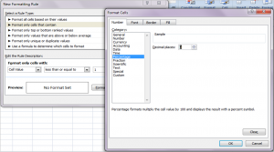
I formatted the column as a number with zero decimal places, to represent salaries. I then applied conditional formatting to check for numbers less than or equal to 1 and format these as percentages.

Conditional format: cells less than or equal to 1

Conditional format: cells less than or equal to 1

This would ensure that if the client entered 30% or 0.3, it would display it as 30%. And if she entered £36,000, it would show £36,000. Remember: while percentages are formatted as percentages, they are stored in Excel as decimals. So 30% is actually stored as 0.3. So the "<=1" check is looking for cells containing a percentage <=100%. Click here for a post all about percentages.

Logic

The next job was to populate column E. I used the following formula to achieve this.

=IF(D2<=1,D5*C5,D5-C5)

This looked in column D to see if it was less than or equal to 1. If it was, then it must be a percentage, so it multiplied the percentage by the base salary to get the uplift amount—in our example, 20% * £30,000, or £6,000. If this condition failed (i.e. a number greater than 1 had been entered), then it would simply subtract the old salary from the new one—in our example, £36,000-£30,000.

Alternate row shading

Alternate row shading is quite useful if you’ve got particularly wide data (lots of columns) and when readers need to scan across individual lines. Bug listings, contact lists etc. I usually use a light yellow shading to help with this, alternating with the default white. In the more recent versions of Excel can be achieved by formatting your data as a table (from the Home tab). But if that's not suitable, or if you're on an older version of Excel, you may still want th feature.

To generate the alternate row shading, I used to insert a new column at A, fill it alternately with 1s and 2s, filter the 1s, shade the filtered rows, then delete column A. The problem with this method is that if you insert a new row some way down, the shading goes a bit awry, leaving two consecutive shaded or unshaded rows.

The better way to do this is to use conditional formatting, and base the conditional format on the row number, or more specifically, whether the row number is odd or even. If the cells you want to highlight start in row 2, highlight rows 2 through n (n being the bottom of your list). Select Conditional Formatting from the Home ribbon. In the first condition, select Formula from the dropdown and type the following into the condition area:

=mod(row(A2),2)=0

Then choose your desired shading through the Format button.

Because the first cell of the range highlighted is A2, it will apply this conditional format to A2, but change the reference accordingly for all of the other cells in the range. The formula itself takes the row number (for row 2, this is 2), divides it by 2 and calculates the remainder (in this case 0). If the remainder is 0 (i.e. the row is even), it will shade it; otherwise, it won’t.

In-cell carriage returns

Excel allows you to wrap text within a cell or within a merged set of cells. But it also allows you to force line-breaks within cells or merged cells.

If you want to create the equivalent of a carriage return within an Excel cell, hit ALT+Enter. The cursor will stay within the cell being edited, but will drop to the next line.

This can be useful when entering regular commentary in a single cell, such as weekly risk updates.

A word of caution though. Usually, these cells behave just fine. But occasionally, if you use the automatic cell height feature, it doesn’t respect these carriage returns and some of your cells’ contents may be hidden. There’s no solution to this beyond manually adjusting the row heights where you see this happening.