PivotTables: the reverse. Creating raw data from a summary

I received an interesting if slightly odd conundrum from Kat the other day. The solution was quite artful, so I thought I'd share.

She had some summary data, each row of which contained a count representing the number of records that row represented. And she wanted to create raw data from that. To anonymise, let's use the following comparable scenario.

Imagine you have a summary of the stock in your warehouse. Each row contains the stock item's ID number, its name, its description, its location together with a count of how many of these items are located there. Kat wanted to create a dataset that contained one record for each individual item, each row containing all of the above details with the exception of the count.

Let's say the source data is in a sheet called Source, and the new dataset will be created in a sheet called Target within the same workbook.

The first job was to work out how many rows we'd need in our target dataset. Easy: that's just a sum of the count column in the source. The source had 248 data rows, and the target would need 438. So in my Target sheet, I put the numbers 1 through 438 in column A.

The aim would be to keep the rows in the same order, so the first few rows of the target would represent the stock in row 1 of the source, followed by rows representing the stock in row 2 of the source etc.

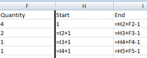
So in the Source sheet, I needed to figure out the start and end rows in the target that each summary row in the source represented. Row 1 had a quantity of 4, row 2 a quantity of 2. So summary row 1 would be represented by rows 1 through 4 in the target; summary row 2 by rows 5 and 6. Etc.

To do this, I created two columns, one to store each of the start and end dates. We manually type a 1 for the start position of row 1. Its end position is the sum of the quantity and its start position, less 1.

We also needed to create the serial number of the row in the source. But we subtract 1 from this number. So the serial numbers of the rows in the source run from 0 through 247. More on why in a moment.

In the target, we insert a column that will contain the source row number that the row will represent—the crux of the challenge, if you will. Let's call this column "Source Row". And we can manually populate the first row of this with a 1.

Now here's the important logic that goes into the target rows. We look up the previous row's Source Row in the amended source row number just mentioned. And when we find it, we'll bring back that row's start position. If that number is greater than the current target row's serial number, then our Source Row reference should be the same as the row above. But when this condition fails, it should increment by 1.

Or in other words, if the start position of the previous row's summary row is greater than the serial number of the row we're on, then we should continue referencing the same source row as did the previous entry. Otherwise, let's increment by one. And in Excel:

=IF(VLOOKUP(B3,Source!$G$2:$H$249,2,0)>A4,B3,B3+1)

Copy that down and you have the serial numbers of the rows that you need to draw data from: four 1s, followed by two 2s, a 3, a 4 etc.

This can be used as the basis for a VLOOKUP to bring back the data itself from the source:

=VLOOKUP($B3,Source!$A:$E,2,0)

Here's a link to the file.

• Tweet