Ever right-clicked and dragged? Start now

There are some things that we do intrinsically. And there are some that grate.

When left-clicking your mouse, you're happy to drag. You might want to select a block of cells, highlight a range of text or group select a bunch of objects.

When right-clicking your mouse however, you never drag. It's not the done thing. Instead, you expect a little pop-up menu to appear inviting you to do something to the thing that you've selected.

But there is one specific time when right-clicking can be accompanied with a drag to achieve some wonderful results. But here's a word of warning: it will feel as odd as putting your socks on in the opposite order. (With respect to socks, try it. Go on.)

Type "January 2012" in cell A1. Now hover over the bottom-right corner of that cell and your cursor will turn into what looks like a plus sign.

If you left-click and drag all the way down to A12, then the column will auto-populate with February 2012, March 2012 […] December 2012. Rather neat. Excel does the same with days of the week and dates.

Now instead try doing exactly the same action, but instead of holding down the left mouse button, hold down the right one. It'll feel very odd, as likelihood is you'll never have dragged in that way before.

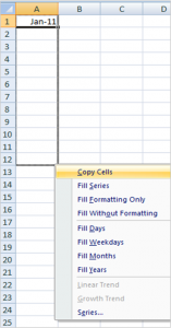
Drag the corner of cell A1 all the way down to A12. Let go of the right-click and you'll be presented with a pop-up menu.

You're given the option of doing the following tasks:

  • Copy Cells: This will simply copy cell A1 down the column. (You probably didn't want to do this. If you did, then CTRL+C, CTRL+V would work just as well.)
  • Fill Series: This will replicate what would have happened had you left-click-dragged instead. It will use its intelligence to auto-fill the series.
  • Fill Formatting Only: This acts the same as Format Painter. (If you wanted to do this, you'd probably choose to use Format Painter instead, right?)

But then it gets interesting. You're presented with some options that are simply delightful.

  • Fill Days: This will fill with sequential days. So if A1 contained 1 January 2012, it will fill through to 12 January 2012
  • Fill Weekdays. Oh hello! This will skip weekend days. 2, 3, 4, 5, 6, 9, 10, 11, 12 13, 16 January. Neat.
  • Fill Months: 1 January 2012 in A1 will fill with the first of each month thereafter. Cleverly, 31 January 2012 will fill with the last calendar day of each month. Beautiful.
  • Fill Years. You get the picture.

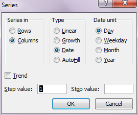
If these options aren't sufficiently varied, then hit "Series…".

This gives you a range of other options, the most useful of which is the step value. If you change this to -1, it will do everything backwards. So you can make it fill with the last day of each calendar month, but going backwards in time. Or choose a step value of 2 to show every other weekday.

The function doesn't only work for dates. You can also use it for numeric series.

So go on. Have a play. And try to get used to right-clicking while dragging.

PureText: the paste-as-text shortcut

Last year, I was looking for a tool that could shortcut the "paste as values" command. My requirement fell outside of Excel – I wanted it to paste into WordPress, MS Word, into Google Mail messages etc. I never even thought of using such a tool in Excel.

After a brief search, I found PureText. It is without doubt the neatest piece of software I've installed in the last few years. And it's free.

It's simple. It launches in the background when you start your machine. And the only thing it does is create a shortcut that pastes whatever's sitting on your clipboard as plain text.

So to copy something, you hit CTRL+C in the usual way. But to paste as plain text, instead of hitting CTRL+V, you hit Window+V. (The Window key is present on most non-Mac keyboards, somewhere to the left of the space bar.)

As well as working in the above-mentioned packages, it's also sublime when it comes to Excel. It bypasses the two mouse clicks that you'd usually need to paste values.

If you're a fan of the keyboard shortcut, then this app's just for you.

Don’t over-engineer when industrial strength is not warranted

I would estimate that 80–85% of my spreadsheets are throwaway. I create them for a specific purpose: to understand some data; to create an import file for one-off use; to prove someone wrong. (Ha!) After its creation date, I'll never use the spreadsheet again.

The other 15–20% of the time, I'm creating a spreadsheet that will last: a model that will be used to run scenarios; a template for analysis month-on-month; a risks and issues register.

Before you set out developing a spreadsheet, it's important to understand which of the above categories your efforts are likely to fall into. Are you creating it to address a burning issue that will be gone tomorrow? Or are you creating a piece of the furniture that needs to stand the test of time?

If you're doing the former, your formulae don't need to be particularly efficient. Error messages don't need to be hidden. Data doesn't need to be streamlined. And exceptions don't necessarily need to be dealt with.

It's easy to adopt a purist mentality, and make your spreadsheet sing and dance at every turn. But if you don't have to, don't bother. Life's too short.

On the odd occasion, one of the spreadsheets you think is temporary becomes strategic and long-standing. (Every week, I use a spreadsheet that I created in 2004 that I thought would be used once.) If this ever happens, you can rewrite or re-jig it in less time than the time you'll have saved cutting corners on the other ones.

Dating in the new year

Some people in the office are whinging about the fact that typing a December date without appending the year defaults to storing it as a 2012 date. They are of the view that Excel should know that they meant December 2011.

You see, if you type a date without bothering with the year, Excel will assume that you mean the current year. So type "12 December" today, and it will store this as 12 December 2012.

I questioned what logic Excel should use. Should it start using the current year in March? June? October? They couldn't answer.

While the behaviour can be a bit annoying early in the new year, there is no better suggestion out there. Maybe Excel ask each user a few questions about what they use Excel for ("do you bill in arrears or advance?") to determine the default behaviour. Or not.

So deal with it.

The odd syntax of the COUNTIF function

My friend Sharon yesterday was trying to get her head around the COUNTIF function. Its syntax is odd, so I sympathise. Here's why.

COUNTIF takes two arguments: a range and a condition.

COUNTIF(Range,Condition)

The range is the thing that you'll count a subset of. The condition is used to evaluate whether or not to count each entry in that range. If you have a range containing the values 1, 2, 3, 4 and 5, a condition of greater than or equal to two will yield a count of four, for example.

The range is easy to specify. It works like any range that you'll find in any formula. Use dollars or don't, it's up to you.

The condition is a little more tricky. While I kind of understand why, most people find it odd that the condition must be encased in double quotation marks. So the above condition would necessitate ">=2", including the quotes

=COUNTIF(A:A,">=2")

Not encasing it in quotes would leave symbols that can do dangerous stuff unrestrained in the middle of formulae, which would be tantamount to madness. But on the other hand, I don't think I've ever seen such behaviour in other walks of programming. It's almost as if you want it to print: >=2

It gets even more odd when you need to put arguments into the condition. For example, instead of referring to a 2, you may want to refer to cell A2:

=COUNTIF(A:A,">="&A2)

This concatenates the value of cell A2 on to the end of the ">=" to form the inequality.

Hope this helps in your counting.

Saving a fixed-width import layout

Excel has an in-built ability to import fixed-width text files. If you try to open a text file, a wizard will appear asking whether it's fixed-width or delimited.

Delimited files are easily processed. With fixed-width files, Excel has a go at figuring out where to insert the column breaks, but more often than not, you'll have to add some, delete others and move some more to get the desired result.

  • To insert a break, just click where you want it
  • To move a break, just drag it to where you want it
  • To delete a break, double-click it.

The frustrating part about it all is that there's no way of saving the layout that you've defined. If you're importing files of the same layout time and time again, this can be a pain.

But there is a solution.

Create a new workbook containing two sheets. One will house the raw data; the other will split it into columns.

Copy your raw data into the top of the first sheet using the traditional copy/paste method. This will all be stacked up in column A.

In the second sheet, we're going to create a frame for separating the data out into its constituent parts.

In row 3, put your column headers. In row 1 put that column's start position in the file. And in row 2, put the length of the field.

Now we'll use the MID function, together with dollars to hold our references, to put data in row 4.


You only need to create the formula in cell B4. Once you've done that, copy it across to the right-most column. Then copy that row down to cover as many records you copied into the original sheet.

I use a spreadsheet just like this regularly, calling it Template. And I pin it to my Excel Recent Documents list so that it's always only two clicks away.

Danger: copying and cutting in a filtered range

If you're cutting or copying content from a filtered range, beware. Here are some behaviours that may catch you out.

First of all, copying.

  • If you copy from a filtered range, Excel will only copy those cells on display. Which is as you'd probably expect
  • When you paste them, however, they will paste into a contiguous range. So if rows 4 and 7 are showing from your filtered range, and you copy copy these two rows to the top of a brand new sheet, the contents of rows 4 and 7 will appear in rows 1 and 2 of your new sheet
  • But if you instead try to copy the contents of a filtered column into another area of the filtered range, you'll get in a mess. So if you try to copy filtered cells A4 and A7 into column B, you'd highlight B4 and paste. But this would paste into B4 and B5, B5 being a hidden unfiltered cell. Very odd.

Now let's look at cutting, a completely different kettle of fish.

  • If you cut from a filtered range, Excel will cut everything in between the top and bottom of your selection, including those intervening cells that are hidden because of filtering.
  • So if you cut cells B4 to B7 (what looks like two cells given the filter hiding B5 and B6), and paste it to the top of a new sheet, the top four cells will be populated (with the contents of B4, B5, B6 and B7)
  • If you instead paste them into column C, then they will paste beautifully.

It's not intuitive. And it's caused me a lot of issues in the past. So be aware of what's going on. And make sure your wits are about you when you're copying or cutting in close proximity to a filtered range.

CLEAN

Summary

The CLEAN function in Excel is a little-known function. As its name suggests, it cleans up text. Or more specifically, it removes all non-printable characters from text.

So wherever you see one of those ugly characters that appear as a square, this is your function. It also removes in-cell carriage returns, which saved me a lot of pain today.

Syntax

=CLEAN(Cell)

Cell is the cell containing the text string you're looking to clean.

How to think about sorting across multiple fields

Some people struggle to get their heads around sorting when more than one field is involved. Below is the best way to think about sorting in these circumstances.

  • First, group everything by this field
  • Within the records with the same value above, group by this field
  • Within the records with the same value above, group by this field
  • Etc.

So if you want to have records within each geography appear together, within which you want to group by business unit and then sort by surname, that is the order in which the fields should appear in the sort order box when you select Custom Sort.

  • Geography (A–Z)
  • Business unit (A–Z)
  • Surname (A–Z).

Cross-sheet data validation

One of the annoying limitations of Excel is that Data Validation does not work from one sheet to another. If you have a list of items that you want to use as a pick list for a specific cell, the cell and the list need to be in the same worksheet.

But apparently not. If the list is a named range, and you refer to that named range in the Data Validation, then it can sit in a different worksheet.

Thanks to Lee Smyth for this one.