First: what is Conditional Formatting?
Conditional Formatting is a feature that allows you to change how a cell looks based on the contents of your workbook. You may have a cube of random numbers, and want to shade everything over 0.8. Or you may have a list of employees, and want to embolden those that earn more than £50,000.
Conditional Formatting has been made rather daunting since the launch of Excel 2007.
In the days before 2007, there was a single Conditional Formatting menu option, from which you could do whatever you needed.
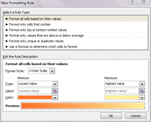
The newer version comes with Data Bars, Color Scales and Icon Sets. There's lots of fun to be had in those areas. But 99 times out of a hundred, what we really want is to define the rules ourselves.
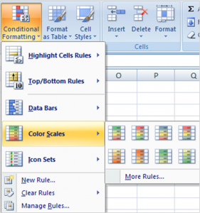
And this means that the bottom three menu items are all we need:
- New Rule…
- Clear Rules
- Manage Rules…
If you know how to use the New Rule feature, then the other two become straightforward. So let's dive in. First, highlight the area that you want to be formatted. And on the Home ribbon, hit the Conditional Formatting button in the Styles area.
Again, the pop-up is littered with stuff that you're unlikely to use. Almost always, I resort to one of two menu items here:
- Format only cells that contain
- Use a formula to determine which cells to format.
The first of these options allows you to format each cell based on its contents. The latter allows you to format each cell based on the contents of others.
Format only cells that contain
This one's relatively straightforward.
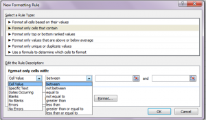
The first dropdown allows you to select attributes of the cell that you want to base your formatting on.
More often than not, you'll choose "Cell Value" here. The Date option can be useful, but otherwise I rarely venture beyond the default.
Once selected, the second dropdown is self explanatory. You select the conditions that need to be met for the formatting to kick in.
Then you select the formats that you want to show when the conditions are met (a richer set than was included in earlier versions of Excel) and you're done.
You can add extra Conditional Formats to allow different scenarios to show different results. Or to allow different cells to be formatted in a multitude of ways. You may, for example, colour numbers under 0.2 green, and those over 0.8 red.
Use a formula to determine which cells to format
This one uses the basics of the above, but takes it to the next level. The key here is that you can format cells based on the contents of other cells. So you can shade an entire row based on the associated value in column K. Or you can insert an upper border if the reference number of the row is different from that in the row above.
(This latter example is useful in visually separating groups of rows. So let's do it.
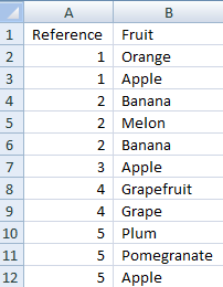
Let's say I have a sorted list of unique reference numbers with an associated list of fruit.
And I want to insert a rule (or a line, to those of more modest age) in between the 1s and the 2s; the 2s and the 3s and so on. But I want the rule to go across the entire row, not just in between the cells of column A.
To do this, I first highlight rows 2 through 12. Note that the uppermost and leftmost cell highlighted is cell A2. This will appear in the little box above the column A title, just beneath the Clipboard area of the Home ribbon. This is important to note.
Just as before, select the New Rule option from the Conditional Formatting option. But this time, select "Use a formula to determine which cells to format.
Here, you are being invited to type a formula whose answer will be either TRUE or FALSE. If TRUE, then the format will kick in. Otherwise, it won't. It's as simple as that.
In the Formula bar, type the following:
=$A2<>$A1
The formula that you type should relate to that uppermost, leftmost cell, in this case A2. But you should use dollars to ensure that the formula is relevant to the other cells that are being given the formats.
In the above formula, we're comparing the value of A2 with the value of the cell directly above it. If they are different (i.e. the reference number has incremented from that in the previous row), then the formula is true, and the conditional format will kick in. Otherwise, it won't.
A dollar has been placed before each of the references to column A to ensure that the conditions that refer to columns B, C, D etc. still refer back to the values in column A. That is, the only things that are ever being compared are the reference numbers. Dollars have not been placed before the row numbers in the formula to ensure that the row references float. So the formatting in row 8 will be based on a comparison between the reference in row 8 and that in row 7, not those in rows 2 and 1.
And lastly, choose your format. In this instance, we choose an upper border as the format of choice. This puts a rule in between rows 1 and 2; 3 and 4; 6 and 7; 7 and 8; 9 and 10.
Give it a try. It really is rather lovely.

 Trouble with formulae? Lookups not going so well? The Wizard of Excel can help. Dan Harrison offers practical tips and examples, as well as Excel training and consulting.


Hi Dan,
i am trying to create an excel spreed sheet to keep all our darting results etc & make it much simpler to complete each week with the selection of rules etc however the one this that is burning my time & confusing me is the following: Can i lock the colour to a row without locking the data within? once all the info is added i have to sort the order of the tables to find out who's moving up the chart & who's dropping down & every time i do that the colours move with the player resulting in blocks of colour rather than every other line which i do simply for easy reading! I would be most greatful if you have a way of locking the colours whilst still allowing me to add info & sort orders without the line colour shifting every time i sort
Kind Regards
Bruce