Olympic ticket allocation spreadsheet: explained

Yesterday, a friend and a Twitter follower (two separate people) asked me to put together a spreadsheet to figure out which Olympics tickets they might have been allocated based on the amount of money that would, they hoped, shortly be whizzing its way out of their respective bank accounts.

So I did. First, I produced a throwaway spreadsheet for Simon. I then went about creating something a bit more strategic.

To make the spreadsheet manageable, I allowed for up to 15 sets of tickets. My understanding is that if you requested four tickets to the Opening Ceremony, you either get them all or you get none.

Fifteen sets of tickets gives 2^15 combinations of tickets offered. Or 32,768.

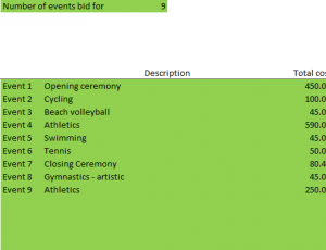
First, the user confirms how many sets of tickets they requested.



The event numbers down the left-hand side are stored as numbers (1–15). There are two features here. First, they all have the following custom number format:

"Event "0

This means that the number can be used in calculations, comparisons etc., but it shows after the word "Event". It's a handy tool.

Also, you'll notice that only the first nine events have event numbers. The cells below Event 9 do contain numbers. But conditional formatting compares them to the number of events entered at the top. If the number is higher than the number of events for which you've requested tickets, then the number is given the following number format:

;;;

The triple-semicolon is a means of hiding the contents of a cell (irrespective of its background colour) while at the same time storing a value therein for calculation and logic purposes. Again, handy.

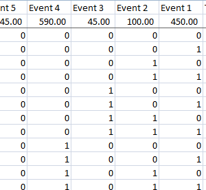
Next, on a second sheet, I had to come up with all 32,768 permutations of tickets being awarded. First, I listed each of the 15 events across the top (listed in reverse order, from 15 to 1). I then created 32,768 rows below, each cell containing a 0 (representing not being awarded that set of tickets) or a 1 (representing being awarded tickets for that event).

With the ticket prices listed across the top in row 2, the following formula was used to establish how much that ticket combination would cost.

=IF(ROW(C3)-2<=2^Bid!$E$1,SUMPRODUCT(C3:Q3,$C$2:$Q$2)+6,"N/A")

The IF statement establishes whether the row in question is valid based on the number of ticket sets selected. For example, if I've ordered four sets, only the first 16 combinations are relevant.

The SUMPRODUCT function takes equally-sized ranges, multiplies together each set of corresponding values and adds these results up. Here, it's multiplying the range of zeros and ones for that row with the corresponding ticket costs. The dollars before the row numbers for the costs mean that when you copy the formulae down, the reference to row 2 holds firm.

Finally, the +6 adds £6, the one-off cost of postage associated with the order. (Criminal!)

Each of these results is then compared with the amount of money taken out of your account, and the exact matches are flagged and numbered.

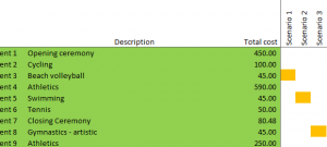
Off to the right of the event data mentioned above, there are 30 thin columns labelled Scenario 1 to Scenario 30. They represent up to 30 ticket allocation combinations, hopefully sufficient. Again, the titles are stored as numbers and conditional formatting hides the redundant ones.

A VLOOKUP is used to bring back the zeros and ones associated with each winning scenario, and conditional formatting hides the zeros (you haven't been awarded that set of tickets) and colours the ones orange (you've been awarded that set).

Hope you like it. Here's the link again.

• Tweet