Excel wordsearch creator

I needed to create some wordsearches recently. So I turned to Excel.

I created two identically-sized grids: a blank one in which I could type the words I wanted to appear in their rightful positions; and another one next to it, which would surround the keywords with randomised letters.

And here's the result. I've shaded the keywords on the right for visual effect. The shading isn't there in the finished product, because that would make the wordsearch a bit rubbish.

The formula of choice is as follows:

=IF(ISBLANK(B4),VLOOKUP(ROUNDDOWN((RAND()*1012)+1,0),Lookups!$F:$G,2,0),B4)

The range in the Lookups sheet lists the letters of the alphabet a variable number of times depending on their propensity to appear in the English language. (E.g. A appears roughly 82 times in 1012, or 8.1% of the time.

Here's the spreadsheet should you want to use it.

Times tables spreadsheet

My daughter's in the midst of learning her times tables. There are various apps out there that can help, but I was after something that addressed a specific need.

I wanted to be able to specify the times tables that she had learnt, and to give her a randomised, exhaustive test containing one question for each one learnt.

So if I selected 2, 3, 5 and 10, I wanted a randomised test containing 48 questions – one for each of the 12 multiples within each of the four times tables.

Not being able to find anything, I decided instead to create something. It can be downloaded here: times tables spreadsheet.

The first tab allows the parent or guardian to choose the times tables that the child has allegedly mastered. Enter the same one twice, and it will double-up the questions for that times table.

The second tab presents the questions in a randomised order to the child. Each question is presented in turn, each question not showing until the child has attempted to answer its predecessor. The child is given a tick or a cross as soon as they answer the question, and at the top of the screen, they're given a live status (at a jaunty angle) showing their progress through the test.

My favourite feature is that the ordering of the questions is randomised, and that random order changes each day you open the spreadsheet. So kids can't get complacent about remembering the order in which the questions appear.

=MOD(10000*A1/DAY(TODAY())/MONTH(TODAY()),1)

(Basically, take a random number between o and 1, divide it by the day of the month; divide it by the month of the year, multiply the result by 10,000 and figure out its decimal remainder. Not proper random; but random enough.)

Here's hoping it helps.

Convert to columns: Carriage-return delimiter

I found out the other day that the carriage return can be used as a delimiter when converting text to columns. This is useful if you have in-cell carriage returns that you want to get rid of. (To do an in-cell carriage return in the first place, you just hit Alt+Enter.)

Highlight your column of data, making sure the columns to its right are empty. On the Data ribbon, hit Text to Columns. Hit the Delimited option, and then check the Other option. Click in the box where you are to type the delimiter and press CTRL+J.

Hey presto, text to columns!

Looking for search substrings in a list of products

Reently, Sam asked me to help with a problem.

I am trying to create a function whereby users of my spreadsheet can type in 1–3 words to search a range of parts descriptions (text entries) and pull up their associated parts numbers and descriptions.

The intent is that they don't know the part number to order or the exact description, so they enter up to three words and it returns all the part numbers with those three words (or some of those words) and the descriptions of thos parts. Hopefully that makes sense.

I don't want it to be case or context sensitive. Is there a way to do this in excel?

Well yes there is.

Let's say that the user enters their search string into cell B3. The first job is to parse the search string, separating it into its three words. To help with this, I've added a space to the end of the search string.

=B3&" "


To find the first word in the string, we have the following formula:

=IF(ISERROR(TRIM(LEFT(B4, FIND(" ", B4,1)-1))),"",TRIM(LEFT(B4, FIND(" ", B4, 1)-1)))

The core of this formula is

LEFT(B4, FIND(" ", B4, 1)-1)

The FIND function is looking for the first instance of a space in the string, and taking one off this value. The LEFT function is bringing back the leftmost characters up to that point. So if the first space appears in character 8, then it's bringing back the first seven characters.

This I've trimmed, which removes double-spaces and any leading or trailing spaces.

And I've wrapped the whole thing in a big IF(ISERROR) clause. This basically says, if this whole formula yields an error, bring back nothing; otherwise, bring back the string.

The formulae for the second and third word are slightly more complex, but follow the same sort of logic.

=IF(ISERROR(TRIM(MID(B4, LEN(B7)+2,FIND(" ", B4, LEN(B7)+2)-LEN(B7)-1))), "", TRIM(MID(B4, LEN(B7)+2, FIND(" ", B4, LEN(B7)+2)-LEN(B7)-1)))

=IF(ISERROR(TRIM(MID(B3, LEN(B7)+LEN(B8)+3, 100))), "", TRIM(MID(B3, LEN(B7)+LEN(B8)+3, 100)))

Note, if the user enters four or more words, the third word formula currently breaks. But that could easily be solved. (I was merely following the business requirements.)

I've then created uppercase versions of each of these sub-strings in H1, I1 and J1.

=UPPER(B7)

In my example, the user has typed in <banana chicken muffin>. For some reason, they're interested in products with any one of those words in them.

Now let's say that we have an inventory list in column F, starting in row 3. In column G, we uppercase that using the same UPPER formula. That means we'll be looking for uppercase words within uppercase strings, so we should be good.

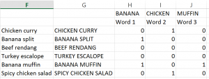
So we have column labels in H, I and J for each of our keywords, and our products appear in the rows. Let's say the first product is chicken curry.

In the intersections (e.g. H3), we put the following formula:

=IF(H$1="",0,IF(ISERROR(FIND(H$1,$G3)),0,1))

This is looking for the word BANANA (the first word of our search string (H1) in cell G3 (which contains CHICKEN CURRY). If it can't find it, it'll return a 0. Otherwise, it'll return a 1.

This formula can be copied down the column and across to columns I and J. So looking for <banana> in <chicken curry> will yield a 0. But searching for <chicken> in chicken curry will yield a 1, as will the search for <banana> against <banana muffin>.

So we now have a matrix of 1s and 0s.
banana

In column D, I've created a simple MAX against the relevant row.

=MAX(H3:J3)

This gives a 1 if that product was found in any of the keywords was found (i.e. the product is relevant) and a 0 if not. And then I've added an incrementing serial number in column E.

=IF(D4=1,E3+1,E3)

So if the current product has been found, add a 1 to the previous serial number. Otherwise, repeat the previous product's serial number.

banana 2


So <chicken curry> has a serial number of 1, <banana split> gets a 2, but <beef rendang> repeats the 2, indicating that the product is not suitable. <banana muffin> is the next one to increment the serial number to 3.

Elsewhere, in column L say, I've put the numbers 1 through 40. And against each, I have a VLOOKUP to bring back the relevant products.

=IF(ISERROR(VLOOKUP(L2, E:F, 2, 0)), "", VLOOKUP(L2, E:F, 2, 0))

This is looking for an exact match of the serial number in column E (our list of sequence numbers) and bringing back the product name (column 2) for the first such occurrence. So against the number 2, it is looking for a 2 in the sequence number, and bringing back <banana split> the first product with that serial number. For number 3, it'll bring back <banana muffin>.

You can hide the redundant product numbers by giving them a Conditional format of <;;;> (without the < and >) if the product field is blank.

Job done!

How to sort your columns

Usually, the requirement is to be able to sort rows in a certain order. But once in a while, I have a need to sort the columns in a dataset. For example, I may want to order my columns in alphabetical order based on the column headers.

It's not too frequent a requirement, but it's sufficiently regularly to warrant addressing, given that Excel has no embedded functionality to do this.

If you have fewer than 16,384 rows of data, this can be done. First, create a new sheet. Copy the contents of your dataset. Go to cell A1 of your new sheet and Paste Special | Transpose. This will flip your data, putting the contents of row 1 in column A; row 2 in column B etc.

Now you can sort your dataset in the traditional way.

And finally, once you're ready, copy the sorted data and use Paste Special | Transpose to get it back into its original location.

Job done!

How to forecast based on a sales pipeline

I work with a company in one guise at the moment, but I don't work with their Sales area. While I have no influence here, I am aware that their sales forecasting is broken.

Having worked in a number of companies in which I've been exposed to Sales, there is often one common yet fundamental issue with their forecasting: sales are considered as binary, things to be won or lost.

While individually this is often the case, it doesn't make for good forecasting.

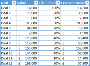
In my view, there is a pretty straightforward way to forecast. In simple terms, you assign a value and percentage to each deal. The value represents the value of the deal in the event that it comes off. The percentage represents the likelihood of the deal coming off.

Sales table

Once done, you calculate the expected value of the deal, which is the product of the two. So, in the above table, if Deal 4 comes off, it'll be worth £183,000. But it only has a 60% chance of coming off. And so the "expected value" of the deal is simply £183,000 * 60%, or else £109,800. Expected value is a statistical term, one that makes sense here.

Now, that forecast is almost certain to be wrong. Deal 4 will either come in at £183,000, or it'll come in at nothing. But if you have enough deals in the pipeline and you are good at predicting likelihood, the above model works at an aggregate level.

For the 12 deals above, if all of them came in, they'd be worth a combined total of £1,492,000. But if you deflate the value of each deal depending on its likelihood to come in, then the expected value of the portfolio is only £685,600.

Take a simpler scenario, one in which there are 10 deals in the offing, each with a 30% chance of coming off, each valued at £1,000,000. An optimistic salesperson might give a sales forecast of £10,000,000. But if your likelihood percentages have been predicted accurately, then only three of those ten deals will come in, and the sales value will be £3,000,000.

I've worked with some companies that have formal definitions for their percentages. (If the legal agreements are drafted and are awaiting signature, then the percentage is 90%, for example. That means even at that stage, one deal in ten is expected to not come off.)

To me, this is the only way to forecast. You need to combine your likelihoods with your values to figure out the expected value of each deal before aggregating.


Where there’s a MIN there’s a MAX

It's an odd one, but wherever you need to apply a minimum in Excel, you'll often find yourself using the MAX formula.

Let's say you need to charge for transactions (stored in cell A1) at a rate of £20 each, subject to a minimum of £3,000, then your formula will read:

=MAX(3000,A1*20)

In this event, if you only have a few transactions (let's say seven), then this will give you the maximum of 3,000 and 140, thus charging the £3,000 minimum.

If you have lots of transactions (237, say), then this will give you the maximum of 3,000 and 4,740, thus charging the transaction fee of £4,740, as it's surpassed the minimum.

So where you see the word "minimum", you might be wise to use the MAX formula.

Always validate the business requirements

George got in touch the other day, in responding to an earlier post on date highlighting. He asked whether there was a way for Excel to automatically insert a row on the left-hand side of a range for each day that passed. So the days would run in reverse order, ascending from right to left. He needed this to allow people to enter hours worked in that day's column.

The key seemed to be the ability to see some other columns while entering the data, columns that would remain static n position at the left-hand side of the spreadsheet. (These columns were the number of hours worked in the last seven days, and the remaining hours to ensure that the worker didn't flout some form of working time directive.)

Now inserting a new column for each day is quite hard. It involves macros and you'd need logic to figure out how many days have elapsed since the spreadsheet was last opened. Indeed, Steve responded (thanks, Steve)

Instead, I suggested using the acres of space available off to the right of the spreadsheet, columns that already exist. And as for ensuring that the two static columns are always visible to the person entering the data, this can easily be achieved with Freeze Panes.

George seemed happy with the response.

You are truly the Excel wizard

In the end, the solution was way simpler than it would have been if the original requirements hadn't been questioned.

Happy days indeed.

Using the text of a formula

I was asked an interesting question by a follower called Frederick recently. He had a column that contained the syntax behind some formulae, but the column of information was stored as text. All of his entries were of the form A*B. So the column might have read:

4*9
3*7
22*13
13*15

None of the formulae had a leading equals sign, and so they rendered as they appear above.

Frederick wanted a second column that contained the answer. So in the above example:

36
21
286
195

I was searching for a way of simply referencing the formulae in a different cell. I hoped INDIRECT might work, but alas not. So instead I used the following

=VALUE(LEFT(A1,FIND("*",A1,1)-1))*VALUE(MID(A1,FIND("*",A1,1)+1,100))

It's a bit clunky, but it does the job given the consistency of the formulae. It takes the value of the stuff to the left of the asterisk, then multiplies this by the stuff to the right.

Linking spreadsheets: don’t do it

Spreadsheets are linked when formulae in one spreadsheet reference cells in another. There are two circumstances in which spreadsheets become linked: consciously and unconsciously.

First, let's deal with conscious linking.

My general rule of thumb on this subject is that spreadsheets should only be linked if two conditions both hold true:

  • The location of the spreadsheets must be static. There must be no emailing them around the place, or moving them from drive to drive; folder to folder
  • There must be an overwhelming reason for the data in the two spreadsheets to be kept separate.

If I do a piece of work for you, I will never link spreadsheets. And I mean never. The ensuing pain just isn't worth it. You see, when the linked spreadsheets are created, everything's dandy. Spreadsheet 1 references some cells in spreadsheet 2. They're both located in the same folder, and everything sings.

But one day, one of the spreadsheets will be moved to a different folder. Or a column that's of vital importance will be deleted.

When you delete stuff that's vital from within a single spreadsheet, it's usually quite easy to spot that it's caused some errors. You'll see a bunch of #REF! values that you can go away and fix.

But when the spreadsheet that's broken isn't even open, then you're in trouble. You delete some stuff from spreadsheet 2 and save it. The following week, you might open spreadsheet 1, and you're suddenly confronted with a bunch of #REF! values. And you have no idea why.

Now for unconscious linking. This happens when you cut or copy stuff out of one spreadsheet and plonk it into another. You might have an entire sheet that you want to hive off, or you may simply cut a chunk of data from a sheet into another workbook.

If that range of data contains any formulae that reference cells outside of that range, then if you click on that cell in its new home, instead of saying:

=B1

your formula will read:

=[Spreadsheet2]Sheet1!B1

And suddenly, you have a problem. As soon as you change Spreadsheet 2, there's a chance that Spreadsheet 1 will break.

So my advice is: kids, don't do it. It's just not worth it.